The sample data are counts of insects caught in 4 types of traps from C. Buddle, 1999. Click "Calculate!" to run this example, or "Clear Inputs" to enter your own data.
You need a Java-enabled browser to run this program. Perhaps your browser has Java disabled?
I have copied the Phylip/DRAWTREE output to a clipboard, so take me to TreeToy!
So far, this calculator is not able to print out a Phylip DRAWTREE string with consensus values for randomized trees. However, by selecting these two options from the More Options... menu:
If you install a local copy of the applet (see below), then you can load and save the contents of a window from or to a file on your machine, without use of the virtual clipboard. These Load and Save buttons next to a window don't work if you are running cluster directly from the web.
Stability analysisThe applet can assess stability of the tree topology under various resampling scenarios, in order to answer the question If I were to repeat this experiment several times, how often would the observed groupings occur?
There are two factors that determine how this analysis is done:
Comparing two trees
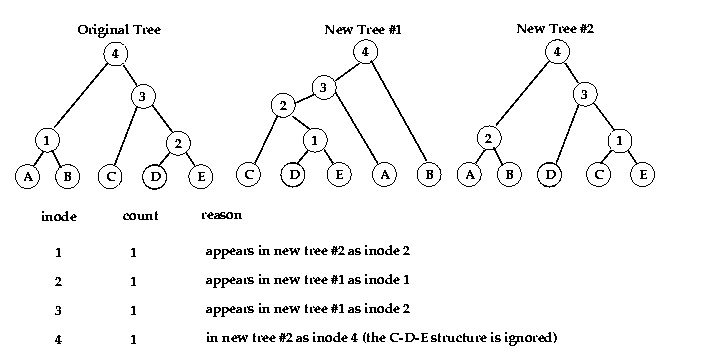
This analysis examines only the topology of the two trees, and ignores branch lengths. Consider an interior node (inode) in a binary tree. The samples which are its descendents (its leaf nodes) form two groups: those descending from the left branch, and those descending from the right branch. We treat this inode's partition of its leaf nodes into two sets as the feature of interest (i.e. for a given inode, we examine only how it splits its descendent samples into two groups, and not the structure within those two groups). So every time we generate a new tree, we check it for inodes that divide the same set of samples into the same two subsets as an inode in the original tree does. The output is a number for each inode in the original tree, giving the number of generated trees in which an inode with the same partition was found. Here's an example:
The calculator accepts input in several formats:
In all cases, if you select the names in "Names Window" option and that window doesn't contain enough names, or if you select the "No Names" option, sample numbers are used as names for unnamed samples.
1     1  1.0 11 4.0 17 7.0 19 4.0 20 2.0
1     32 4.0
2     1  3.0 4  2.0 6  3.0 7  4.0 11 4.0
2     16 5.0 17 5.0 19 4.0 20 7.0 27 5.0
2     32 3.0
extra 2  4.0 4  7.0 6  2.0 11 4.0 16 2.0
extra 32 6.0
Each sample can occupy several consecutive lines. The first number (or name) in a line is the sample number (or name), and the rest of the line is a sequence of (item, abundance) pairs. For example, sample "extra" has an abundance of 4.0 for item 11. Abundances of items not listed for a sample are zero. For example, sample 2 has an abundance of 0.0 for item 5. Distances between samples are calculated using the Euclidean metric. If you select "Data Window" as the location of sample names, then the first "word" in each line is taken as the sample name. The number of spaces or tabs between items is not important, but newline characters are: each line must begin with a sample name or number.
Square Distance Matrix Example (with names):
ridge 0.0 0.1 0.3 0.9
floor 0.1 0.0 0.5 0.6
banks 0.3 0.5 0.0 0.7
other 0.9 0.6 0.7 0.0
The window must contain a number (representing distance or similarity) for each orderered pair of samples. If you select "Data Window" as the location of the sample names, then the name of each sample must appear just before its list of distances to other samples. Here, the distance from sample "banks" to sample "other" is 0.7 If you have similarity data, select "Square Similarity Matrix", and the calculator will obtain distances by subtracting each similari from 1.0 Only the lower triangle of the input is used, and the calculator does not verify that your input matrix is symmetrical and has zeroes (or ones) along the diagonal.
Names and numbers in the window must be separated by spaces, tabs, and/or newlines, but unlike for the Cornell Condensed format, only the order matters! For example, this input is considered equivalent to the previous example:
ridge 0.0 0.1
0.3 0.9
floor
0.1 0.0 0.5 0.6
banks 0.3 0.5 0.0 0.7 other 0.9 0.6 0.7
Upper Triangular Distance Matrix Example (with names):
ridge 0.1 0.3 0.9
floor 0.5 0.6
banks 0.7
other
Lower Triangular Similarity Matrix Example (with names):
ridge
floor 0.9
banks 0.7 0.5
other 0.1 0.4 0.3
Lower Triangular Similarity Matrix Example (without names, with diagonal):
0.0
0.9 0.0
0.7 0.5 0.0
0.1 0.4 0.3 0.0
The window must contain a number (representing distance or similarity) for each unorderered pair of distinct samples. If you select "Data Window" as the location of the sample names, then the name of each sample must appear just before its list of distances to other samples. Here, the distance from sample "banks" to sample "other" is 0.7 (and their similarity is 0.3) The zeroes along the diagonal of a distance matrix, or the ones along the diagonal of a similarity matrix can be present, but if so, make sure to check the "Diagonal Present" option. If you have similarity data, the calculator will obtain distances by subtracting each similarity from 1.0 Only the lower triangle of a square matrix is used, and the calculator does not verify that such a matrix is symmetrical and has zeroes (or ones) along the diagonal.
Names and numbers in the window must be separated by spaces, tabs, and/or newlines, but unlike for the Cornell Condensed format, only the order matters! For example, this input is considered equivalent to the previous example:
0.9 0.7 0.5
0.1 0.4
0.3
Character Matrix: Samples as Rows Example (with names):
7
A B C D E F G
Lake 0 4 0 0 5 0 6
Pond 3 0 0 2 3 3 0
Lawn 1 0 0 2 1 1 0
There is a list of characters for which each sample has a value. In this example, there are 7 characters, each representing the abundance of a different species of insect found in sweep samples at different locations. The first item in the window is the number of characters in each sample. The rest of the window must contain a number for each sample-character pair (even if it is zero), and all numbers for a given sample must appear consecutively. To accomodate the natural layout of this kind of data, this applet now assumes row and column names are present. This assumption can be turned off under the More Options... menu.
If you select "Data Window" as the location of the sample names, then the name of each sample must appear just before its list of character values. The distance between samples is calculated using the distance/similarity measure you choose. Names and numbers in the window must be separated by spaces, tabs, and/or newlines, but unlike for the Cornell Condensed format, only the order matters! For example, this input is considered equivalent to the previous example:
7 A B C D E F G Lake 0 4
0 0 5 0 6 Pond 3 0 0 2 3 3 0
Lawn 1 0
0 2 1 1
0
Character Matrix: Samples As Columns Example (with
names):
7
  Lake Pond Lawn
A 0 3 1
B 4 0 0
C 0 0 0
D 0 2 2
E 5 3 1
F 0 3 1
G 6 0 0
This is the transpose of the Samples as Rows format: the first item is the number of characters in each sample. This is followed by the sample names, if you selected the "Names in Data Window" option, and then for each character, the values it takes in each sample. In this example there are 7 characters, and three samples, namely "Lake", "Pond", and "Lawn". The value of the fifth character for the Lake sample is 5, and the value of the first character for the Lawn sample is 1. As for the Samples-as-rows format, only the order of the data matters.
About the Distance/Similarity Measures
For the Cornell Condensed, Sample-Character, and Character-Sample input formats, you can choose the method for calculating distances (or similarities) between samples.
Distance Measures
The distance between two samples is calculated using their values
for each character, in various ways.For the following table, Xik
is the value of character k for sample i, and |X|
means the absolute value of quantity X.
|
Name |
Distance between samples i and j |
| Euclidean | Square-root of the sum over all characters k of (Xik -Xjk )2 |
| Mean Censored Euclidean | Square-root of (the sum over all characters k of (Xik -Xjk )2/ n ) where n is the number of characters for which at least one of the two samples has a non-zero value |
| Bray-Curtis | (Sum over all characters k of |Xik -Xjk
| ) divided by (Sum over all characters k of Xik + Xjk ) |
| Canberra | (Sum over all characters k of |Xik -Xjk
| / (Xik + Xjk ) ) divided by the number of characters |
(Binary) Similarity Measures
The similarity of two samples is calculated using only the presence
or absence of each character in each sample, where presence means a value
greater than zero for the character. For the following table, the variables
a, b, c, and d mean the number of characters:
a = present in both samples
b = present in sample i, absent in sample j
c = present in sample j, absent in sample i
d = absent in both samples
|
Name |
Similarity of samples i and j |
| Jaccard |
a / (a + b + c) |
| Sorensen |
2a / (2a + b + c) |
| Simple Matching Coefficient |
(a + d) / (a + b + c + d) |
| Baroni-Urbani and Buser | (a + ( ad )1/2 ) / (a + b + c + ( ad )1/2 ) |
If a similarity measure gives a value of S, then the distance
between the two samples is calculated as 1.0 - S
and this will be the value used in the clustering algorithm.
The methods used here are all hierarchical and combinatorial:
The methods differ only in how they calculate the "distance" from one cluster to another:
|
Clustering Method |
Distance Between Clusters A and B (where A was formed by combining cluster A1 with cluster A2) |
| Single Linkage | the smallest distance between a sample in cluster A and a sample in cluster B |
| Complete Linkage | the largest distance between a sample in cluster A and a sample in cluster B |
| Unweighted Arithmetic Average | the average distance between a sample in cluster A and a sample in cluster B |
| Weighted Arithmetic Average | the weighted average distance between a sample in cluster A and a sample in cluster B. The weight assigned to the distance between samples S1 (in A) and S2 (in B) is (1/2)^G where G is the sum of the nesting levels of S1 and S2. (The nesting level of a sample is the number of its enclosing clusters at this stage, in other words, the number of times the sample has participated in a "combine" step.) The effect is to reduce the influence of groups of similar samples, if such are present, on the clustering process. |
| Unweighted Centroid | Cluster A is treated as the centroid of clusters A1 and A2. The distance from A to B is the average of the distance from A1 to B, and the distance from A2 to B, corrected so that A lies on a line joining A1 and A2, in the abstract "metric" space. This is a recursive definition. The distance between a pair of single-member clusters is just the distance between their member samples. |
| Weighted Centroid | like the unweighted centroid method, but reduces the influence of large numbers of similar samples |
| Ward's Minimum Variance | the increase in the mean squared deviation (from a sample to the centroid of its containing cluster) that would occur if clusters A and B were fused |
Note: Output from this program cannot be printed directly. Use the clipboard (or Virtual Clipboard) to copy and paste the contents of the Output window into your favourite word processor.
The program always prints out the clustering algorithm chosen, and the number of samples. By checking the appropriate box on the calculator, you can have it output the:
You can choose to have the program output either similarities or distances, in both the matrix and table output and in the clustering progress output. This does not affect the computations, the distances output for the tree as a text picture, nor the labels output for the Phylip tree output.
The Distance/Similarity Table option shows distances/similarities between pairs of samples in a table. This can be used to verify that your input data is being correctly interpreted.
For example, the sample data produces the following output, if you check the "output similarities instead of distances" option.
From    To      Similarity
========================
PLI     CH      0.88
CI      CH      0.99
CI      PLI     0.88
NS      CH      0.66
NS      PLI     0.62
NS      CI      0.66
CL      CH      0.77
CL      PLI     0.7
CL      CI      0.78
CL      NS      0.73
CT      CH      0.75
CT      PLI     0.71
CT      CI      0.75
CT      NS      0.64
CT      CL      0.76
SI      CH      0.36
SI      PLI     0.36
SI      CI      0.36
SI      NS      0.28
SI      CL      0.29
SI      CT      0.34
SPI     CH      0.51
SPI     PLI     0.51
SPI     CI      0.5
SPI     NS      0.53
SPI     CL      0.51
SPI     CT      0.46
SPI     SI      0.19
SGI     CH      0.49
SGI     PLI     0.49
SGI     CI      0.48
SGI     NS      0.5
SGI     CL      0.49
SGI     CT      0.45
SGI     SI      0.2
SGI     SPI     0.8
For each sample, its name is followed by the distances between it and the samples preceding it. Here, the distance between sample SPI and sample SI is 0.81, and the distance between CT andCI is 0.256667
The Distance/Similarity Matrix option shows the lower triangular matrix of distances or similarities between samples. This can be used to verify that your input data is being correctly interpreted.
For example, the sample data produces the following output, if the "output similarities instead of distances" option is not checked:
Distance matrix:
        CH      PLI     CI      NS      CL      CT      SI      SPI
PLI     0.12
CI      0.01    0.12
NS      0.34    0.38    0.353333
CL      0.23    0.3     0.25            0.27
CT      0.25    0.29    0.256667        0.338   0.24
SI      0.64    0.64    0.64            0.72    0.71    0.668333
SPI     0.49    0.49    0.493333        0.47    0.49    0.54            0.81
SGI     0.51    0.51    0.503333        0.485   0.5     0.506667        0.7025  0.2
For each sample, its name is followed by the distances between it and the samples preceding it. Here, the distance between sample SPI and sample SI is 0.81, and the distance between CT and CI is 0.256667 The formatting is a bit wonky, but it should allow the text to be cut and pasted directly into TAB-aware programs like spreadsheets.
The Clustering Progress option shows the step-by-step progress of the clustering method. The output is a table showing the two clusters joined at each step, and the distance or similarity between them.
For example, the sample data produces the following output, if the "output similarities instead of distances" option is not checked:
Clustering procedure:
Step       A      B    Distance
===============================
1       CI      CH      0.01
2       1'      PLI     0.12
3       SGI     SPI     0.2
4       CT      CL      0.24
5       4'      2'      0.256667
6       5'      NS      0.338
7       3'      6'      0.506667
8       7'      SI      0.7025
At the first step, the samples CI and CH are joined because the distance separating them, 0.01, is the smallest of any pair of samples. At step 2, the cluster formed in step 1, namely "1'", is joined to sample PLI at a distance of 0.12 The "'" is added to cluster numbers to prevent confusion with sample names which might happen to be numbers.
The Tree as Text Picture option draws a tree representing the clustering process. The samples form "leaf" nodes which occur at the right of the picture. Each step in the clustering process is represented by an "interior" node, which has descendents to its right. The calculator also shows a table listing the distances between adjacent nodes.
For example, the sample data yields the following tree:
Tree Topology: (branch lengths ignored)

          +----SGI
     +----+1
     |    +----SPI
+----7
|    |              +----CT
|    |         +----2
|    |         |    +----CL
|    |    +----5
|    |    |    |         +----CI
|    |    |    |    +----3
|    |    |    |    |    +----CH
|    |    |    +----4
|    |    |         +----PLI
|    +----6
|         +----NS
8
+----SI

From    To        Length
========================
1'      SGI     0.1
1'      SPI     0.1
7'      1'      0.153333
2'      CT      0.12
2'      CL      0.12
5'      2'      0.00833333
3'      CI      0.005
3'      CH      0.005
4'      3'      0.055
4'      PLI     0.06
5'      4'      0.0683333
6'      5'      0.0406667
6'      NS      0.169
7'      6'      0.0843333
8'      7'      0.0979167
8'      SI      0.35125
The structure of the tree represents the clustering process: the two descendents of an interior node are the two clusters joined at that point in the process. For example, clusters 2 and 4 were combined to create cluster 5. Although no attempt is made to represent distances in the drawing of the tree, a table is printed listing the actual distances between adjacent nodes. These distances have the property that for any pair of leaf nodes (ie. samples), the distance you get by tracing along the tree from one node to the other, adding appropriate values from the table as you go, is equal to the distance at which the two nodes joined the same cluster. For example, samples NS and CI are connected by the following path:
From    To      Distance
=========================
 NS     6'      0.169
 6'     5'      0.0406667
 5'     4'      0.0683333
 4'     3'      0.055
 3'     CI      0.005
-------------------------
Total Distance: 0.338
The "tree length" between NS and CI is thus 0.338, and this is the same as the distance at which clusters 5 and NS were joined in step 6, as can be seen in the Clustering Progress table.
For the Unweighted Arithmetic Mean clustering method used in the example, this fact can be stated in several ways:
Statements 1 and 2 would be true regardless of which clustering method generated this output. Statement 3 is only true for the Unweighted Arithmetic Mean clustering method.
This statement is not equivalent and doesn't follow from the previous ones:
For the other clustering methods, similar kinds of statements are true and not true.
The Tree in Phylip/DRAWTREE format option outputs a string representing the tree in a way that the Phylip program DRAWTREE can plot the tree in two dimensions. This string can also be used in the TreeToy webpage, as described below. For example, the sample input yields the following Phylip tree:
Tree in Phylip/DRAWTREE format:
(((SGI:0.1,SPI:0.1):0.153333,(((CT:0.12,CL:0.12):0.00833333,
((CI:0.005,CH:0.005):0.055,PLI:0.06):0.0683333):0.0406667,NS:0.169):0.0843333):0.0979167,SI:0.35125);
If you want to look at your tree in a two-dimensional graphical form that reflects tree distances, you can use TreeToy as follows:
Warning: your browser will probably discard the contents of the Clustering output window when you visit TreeToy, so make sure you copy/paste out anything you don't want to lose!
Phylip is a package of free clustering, phylogeny, and data analysis programs produced by Joel Felsenstein et al, and is available for many platforms. You can visit its homepage. The Phylip DRAWTREE program will take a textual representation of a tree (such as can be produced by this calculator), and render it as a two-dimensional graph in various graphics formats, many of which can be printed. If you want to print your graph, consider downloading a version of Phylip.
The Virtual Clipboard lets you paste data into or copy data out of multi-page windows. The ---> VC and <--- VC buttons move data to and from the virtual clipboard. If you see a "Browse" button below, then your browser will also let you copy a file on your machine to the Virtual Clipboard. You can then paste it from the V.C. into the calculator's input windows.
Name of file:
The Virtual Clipboard is Brainless
Is your window full of garbage after pasting? Unfortunately, the Virtual Clipboard knows nothing about file formats, so cutting and pasting directly from an Excel file will fill your window with junk (ie. raw Excel file bytes). You can, however, copy from the open Excel worksheet to a text editor, then save as text in a new file which you can then copy to the Virtual Clipboard. You can also just save a copy of your Excel file in tab-delimited text format, and copy that file to the VC. The point of the VC is just to help work around the limitations on window size in Netscape, MS Explorer, and probably other browsers.
Some browsers limit the size of text windows, so this program allows for bigger input and output using multiple pages. Each page is limited to around 10000 characters. To see if you have filled a page, try typing more characters at the end of the window. When you use your system's copy/paste functions to get text in and out of this program, you have to do so one page at a time; the program has no control over this.
Here are some problems you might encounter (there are doubtless many others - please let me know!):
The clustering functions are slightly-modified Java translations of FORTRAN code by Fionn Murtagh, available from the statlib S-plus archive as multiv. Free use and redistribution are permitted for non-commercial purposes.
The DRAWTREE textual tree format comes from the Phylip package by Joel Felsenstein et al. My thanks to them for making it free.
Thanks for motivation and feedback to Jim Hammond, Mark Dale, John Spence, Greg Wilson, Curtis Strobeck, and Charley Krebs.
This is free software.
For why software should be free, see http://gnu.linux.ucla.edu/philosophy/why-free.html
For other free ecology programs, see http://www2.biology.ualberta.ca/jbrzusto
This Java and HTML/PHP web page is by John Brzustowski (junkjbrzusto@ualberta.cacaca but removing the obvious parts). You can email me comments or criticisms. Although I strive to ensure the correctness of these programs, you use them entirely at your own risk. There is no warranty!
Installing CLUSTER on Your Machine
If your connection to this server is slow, you can get your own copy of the program:
The virtual clipboard can only be used in conjunction with a web server. See above before deciding to try the following. Your webmaster can set up your server to allow you to use the virtual clipboard as follows:
The zipped java source for this applet is here.